Filters are a powerful tool in Excel that can help you quickly organize and analyze large data sets. With filters, you can easily find the information you need without having to manually search through thousands of rows of data. In this blog post, we’ll discuss how to filter in Excel so that you can take advantage of their many benefits.
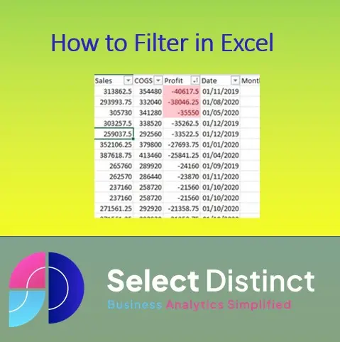
You can download this sample workbook to follow along
Sample Excel Workbook
Setting up filters in Excel
First, let’s talk about setting up your filter:
To set up a filter on an Excel spreadsheet,
select the column or columns that contain the data for which you want to create a filter.
Then click on “Data” at the top menu bar and then select “Filter.”
There is also as Advanced Filter (which allows more complex filtering).
How to filter in Excel, step by step
Now let’s look at how we actually use our newly created filters:
Filtering works by allowing us to view only certain results based on our criteria
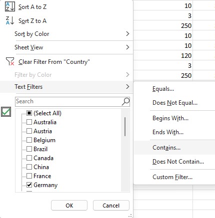
Lets start by filtering the data for all records in Germany,
click on the arrow in the Country column,
click select all which by default will be ticked, you need to deselect.
Then scroll down to Germany and click the tick box there to filter records to just Germany.
Note that you can select multiple options at the same time
Now, with Germany still selected, you can select Small Business in the Segment column and both sets of criteria will be applied

Filtering partial text
Remove all the filters
Now on Country, select Text Filters and then in the options select contains
then enter ‘land’ and click OK
All countries in the data that contain the four letters are filtered, including Ireland, Poland, Switzerland, Thailand and even Netherlands (note it doesn’t have to end in land)
Sorting using a filter column
Clear all the filters
Click on the profit column and sort smallest to largest
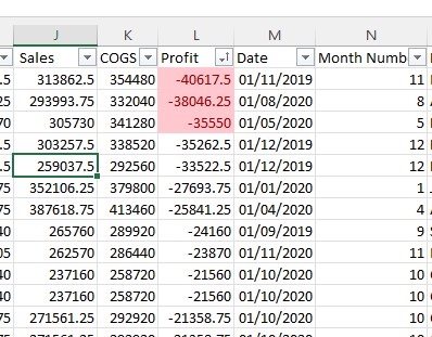
Then highlight the cells with the biggest negatives and set the format to be red background
Now sort the profit column largest to smallest and highlight some of the largest profit values with a green background
How to Filter by colour excel
With some cells now having coloured cells we can use this to filter for colours
Click the filter in the Profit column, filter by colour and select the colour you want to filter, either red or green in this example
This can be very useful if you have reviewed the data and want to highlight particular values, simply colour code them and filter all the colours when you have finished
More filter options
Number fields can be filtered using a wide range of options
Click on units sold, and select number filters then select top 10
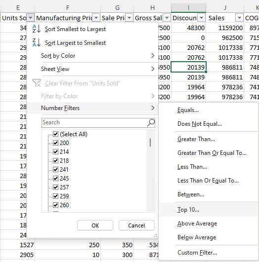
Instead of single condition like above mentioned scenario – say looking specifically ‘Greater Than’ 10 – users may choose multiple conditions such AND/OR statements e g : show me all entries between 5 & 20 OR even further refine search parameters involving text strings too like finding exact matches against specified keywords etc… All these tasks become possible thanks its advanced filtering capabilities provided here making life much easier compared to manual searching
Now you know how to filter in Excel
Watch our You Tube Video – How to Filter in Excel
Subscribe to our channel to see more Excel Timesavers
Select Distinct YouTube Channel
Our Business Analytics Timesavers are selected from our day to day analytics consultancy work. They are the everyday things we see that really help analysts, SQL developers, BI Developers and many more people.
Our blog has something for everyone, from tips for improving your SQL skills to posts about BI tools and techniques. We hope that you find these helpful!