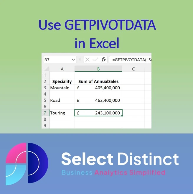
Using the GETPIVOTDATA Function in Excel to add flexibility to your Data Analysis & Reporting
What is GETPIVOTDATA and How Can It Help You?
The GetPivotData function in Excel provides users with the ability to return specific data points from a pivot table, Think of it like a specialised lookup mechanism that can find an aggregate value across many dimensions
Having the ability to extract a key value from a pivot table and return that into a specific cell enables a great deal of flexibility in your reporting
If you want to know how to create a pivot table, here is a short guide
How to create Pivot Tables in Excel – Select Distinct
How to Use GETPIVOTDATA in Excel
Start with a pivot table
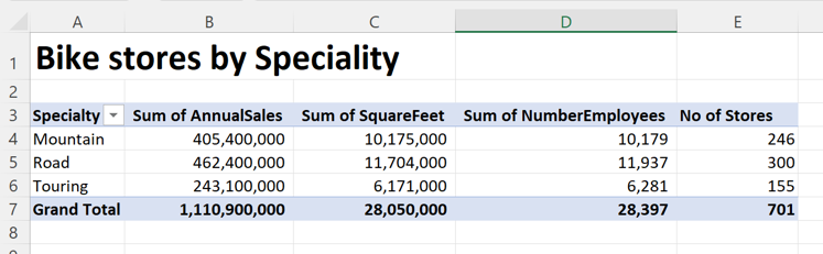
In this example we will return the total annual sales for each of the speciality bikes
Go to a new Worksheet and click in a blank cell
Press equals (=), then select the cell in the pivot
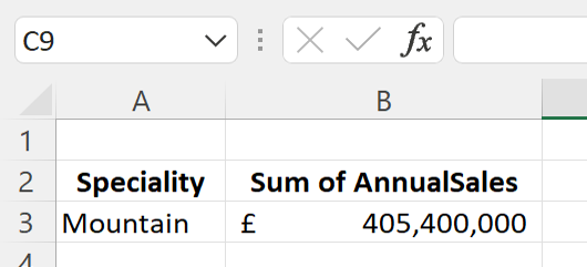
Here we click on the Sum of Annual Sales for the Mountain bikes
Excel generates a GETPIVOTDATA formula for you and returns the value to the cell you selected
=GETPIVOTDATA(“Sum of AnnualSales”,’Summary PIVOT’!$A$3,”Specialty”,”Mountain”)
Press enter and the value is returned to the cell
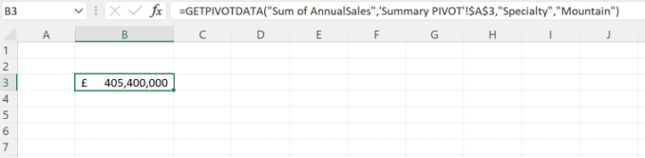
The value for the Total Sales is shown in cell B3
You can now select individual values from the pivot table and place them anywhere you like
Adding More Flexibility
To make better use of the getpivotdata formula
Add Headers to the Row and Column to explain what the data is
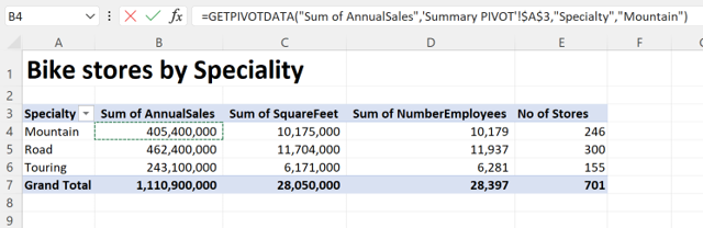
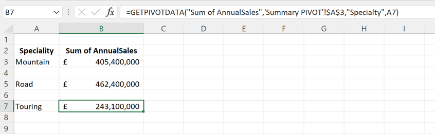
You can amend the formula with Column or row headers and excel will find the intersect of those
=GETPIVOTDATA(“Sum of AnnualSales”,’Summary PIVOT’!$A$3,”Specialty”,A3)
Here we have changed the reference from being a hard coded “Mountain” to the value in cell A3 (Mountain)
You can now copy and paste the formula to create other extracted values
Copy and paste the row down to another row and check the speciality reference
The formula will now pick up the intersect of the row and column in the Pivot table
Understanding the Formula Syntax
GETPIVOTDATA([data_field], [pivot_table], [field1, item1, field2, item2], …)
=GETPIVOTDATA(“Sum of AnnualSales”,’Summary PIVOT’!$A$3,”Specialty”,A3)
The GETPIVOTDATA function has the following components:
1.Data_field (mandatory) – This is the pivot table ‘Values’ field, in this case “Sum of AnnualSales”
2.Pivot_table (mandatory) – The reference of the pivot table, usually the top left call value of the pivot table. E.g. ‘Summary PIVOT’!$A$3
It can also be a range of cells, or named range of cells in a pivot table.
3. Field1, Item1, Field2, Item2 (optional argument) – 1 to 126 pairs of field names and item names that define the data. The pairs can be in any order. Field names and names for items other than dates and numbers need to be enclosed in quotation marks or be a call reference
e.g. Field = “Speciality”, Item = A3 or “Mountain”
Advantages of the GETPIVOTDATA function
Some of the benefits of GETPIVOTDATA in Excel are:
– It allows you to extract data from a pivot table based on the structure and names of the fields, not the cell location. This means that the function will still work correctly even if the pivot table changes in size, layout, or position
– The formulas easier to read and understand, as you can use the actual names of the fields and items instead of looking up their internal names or cell references
– You can use calculated fields or items and custom calculations in pivot tables, as well as dates and times
– It can be combined with other functions, such as DATEVALUE, to prevent errors or format mismatches when using dates in pivot tables
It can be very useful if you want to generate a summary page which pulls data from a range of different pivot tables, maybe across many worksheet tabs. By pulling out the key data points from the intersects on the pivot tables you can draw attention to important points
Subscribe to our channel to see more Excel Timesavers
Select Distinct YouTube Channel
Our Business Analytics Timesavers are selected from our day to day analytics consultancy work. They are the everyday things we see that really help analysts, SQL developers, BI Developers and many more people.
Our blog has something for everyone, from tips for improving your SQL skills to posts about BI tools and techniques. We hope that you find these helpful!