This quick guide shows you how to create pivot tables in Excel
What is a Pivot Table?
Pivot tables are an incredibly powerful tool in Microsoft Excel, providing a dynamic and intuitive way to analyse, summarize, and manipulate large amounts of data.
By using a drag-and-drop interface, users can quickly and easily create summaries from complex datasets and organize data into meaningful visual representations such as charts and graphs.
Pivot tables can also be used to quickly filter data or perform calculations such as sums, averages, and counts. In addition, pivot tables can be used to identify and highlight trends in the data, and can even be used to create interactive dashboards for data exploration and reporting.
How to create a pivot table in Excel
Open an Excel workbook which has a data table you want to analyse
Go to the Insert Tab
Select
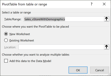
Select the table or range of cells you want to analyse
Click OK
If your data table is defined as a table in Excel, you can just enter the table name
If it is not defined as a table, you can enter the range
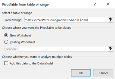
The dataset is then loaded into the pivot table definition
Designing the Pivot Table layout
You can now start to design the pivot table using Columns, Rows, Values and Filters
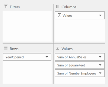
Rows
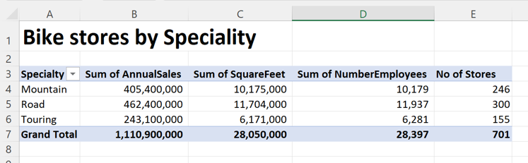
To start with, its good to select categorical fields into the rows, here we are using the Year Opened field to provide a summary row for each year
Values
This is where we define which fields we want to summarise, in this example we want to see totals for Annual Sales, Square Feet of each store location and the total number of employees
Columns
We have set the individual values to appear in columns, but these can also be moved to rows to show a different perspective
Filters
Filters can provide the ability to filter out specifics, or focus in on a single area by setting filter for a field or a number of fields as required
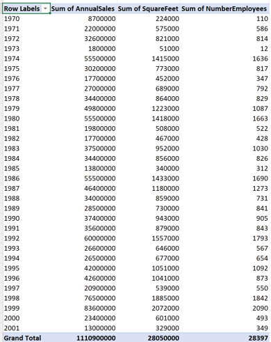
This gives us this Pivot Table
Applying Filters and Sorting in a Pivot Table
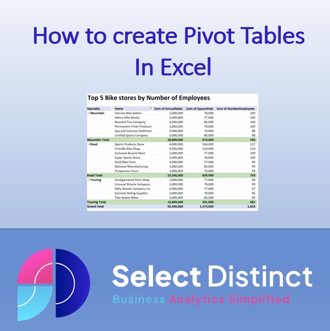
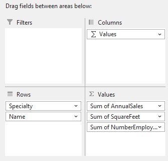
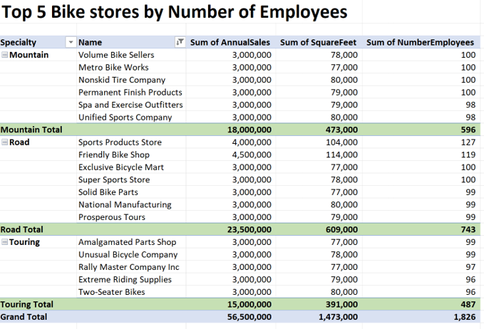
We now want to show the Top 5 Bike Stores by Number of Employees
Drag Speciality and name to the Rows and remove Year Opened
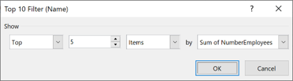
We only want to see the top 5 stores by number of employees
To do this, right click on any of the values in the Name column, then use these settings
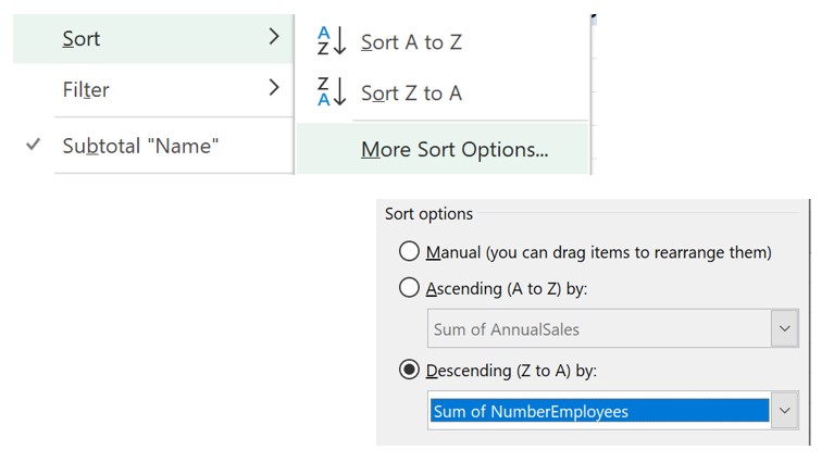
It is also good practice is showing a top 5 to also sort by the same metric, we want the sort order to reflect the order of the top 5 filter
Right click on the Name field, sort, More sort options and sort descending by Sum of Number of Employees
Improve the appearance
Set the number formats to have comma separators
Select anywhere on the pivot table, then on the ribbon select design
Then choose tabular form
Or experiment to find your own preferred style, Excel has a wide range of settings to allow you to get creative on the design
Here is the result of changing a few options for number formats, and shading the subtotals
Now you know how to create pivot tables in Excel
Once you understand how Pivot Tables work, you unlock a whole range of analysis that is fast, robust and flexible
Watch this space for more advanced Pivot Tables
Subscribe to our channel to see more Excel tips and timesavers
Select Distinct YouTube Channel
Or find other useful Excel timesavers in our Blog
Explore more guides in the Business Analytics Blog